Introduction
In the automotive industry, noise, vibration, and harshness (NVH) reduction technologies have become a key factor in determining vehicle quality, and accordingly the importance of stiffness prediction techniques for rubber anti-vibration components has been continuously increasing. Rubber components such as engine mounts, suspension mounts, and bushings exhibit nonlinear behavior under both dynamic and static loading conditions, which arises from the inherent incompressibility, large deformation capability, and nonlinearity of rubber materials. Therefore, in the design and analysis of automotive rubber components, it is essential to define material properties based on hyperelastic models.1
The stress–strain curves of rubber materials are influenced by various factors such as test conditions, initial load offsets, noise, and irregular strain intervals, and these uncertainties directly cause problems in the convergence and coefficient stability of hyperelastic model fitting. In particular, the raw data, due to initial offsets and non-uniform spacing, tended to produce divergence or negative coefficients when fitting higher-order hyperelastic models. Abaqus Evaluate does not provide sign constraints on the coefficients and therefore frequently exhibits such issues,2 whereas Marc Experimental Data Fit enforces sign constraints through the Positive Coefficients option and thereby maintains physically reasonable combinations of coefficients.3
To compensate for the irregularity of the raw data, preprocessing schemes such as zero-setting data and simply preprocessed data were employed. Zero-setting data corrects the zero point of the raw data by removing the initial offset, while the simply preprocessed data rearranges the strain values at uniform intervals to generate continuous data. These differences in preprocessing affected not only the stability of the Ogden coefficients and the fitting results of each solver, but also the predicted stiffness and convergence range in product-level finite element analyses.1
In this study, uniaxial and equibiaxial tensile tests were conducted to obtain the fundamental material properties of the NR/BR, and the stability of the third-order Ogden model coefficients was analyzed for the raw data, zero-setting data and simply preprocessed datasets. In addition, the same data sets were applied to Abaqus and Marc, respectively, to compare differences in the solver algorithms, and the derived coefficients were implemented in finite element models of the actual product to validate their predictive performance. Finally, in view of industrial applicability, the feasibility of a lightweight fitting procedure based on Excel Solver was also discussed.
Experimental
The large-deformation behavior of rubber materials is described by the deformation gradient tensor F, and the Right Cauchy-Green tensor4
The deformation state of rubber materials can be expressed in terms of the principal stretches (λ1, λ2, λ3) and the strain invariants I1, I2 and I3, are as follows5
Since rubber is nearly incompressible, the condition λ1, λ2, λ3=1 holds. The stress is calculated by differentiating the strain energy function W with respect to the deformation gradient,4
And the nominal (first Piola-Kirchhoff) stress P and the true (Cauchy) stress σ are defined by the following relations.
The Neo-Hookean model is the simplest hyperelastic model based on the first strain invariant I1 and is defined as follows.6
This model exhibits adequate accuracy in the small-strain regime but shows clear limitations under large deformations.
The Mooney-Rivlin model combines the first and second strain invariants I1 and I2 and is expressed as6
It provides better performance than the Neo-Hookean model in shear deformation and in the initial nonlinear region, but its accuracy deteriorates at large strains.
The Ogden third-order model used in this study is a principal-stretch-based model and is given by6
• μi : material parameter controlling stiffness
• αi: material parameter controlling the nonlinear stiffness response
Where N=3 for the third-order Ogden model.
The Ogden model reproduced the experimental data well under both uniaxial and equibiaxial large deformations and was therefore the most suitable for the present study.
To obtain the raw data, two test modes were carried out. All tests were performed under room-temperature conditions, and the NR/BR specimens were stabilized by 2-3 cycles of preconditioning before measurement. The geometries of the uniaxial and equibiaxial tensile specimens used in this study are illustrated in Figure 1.
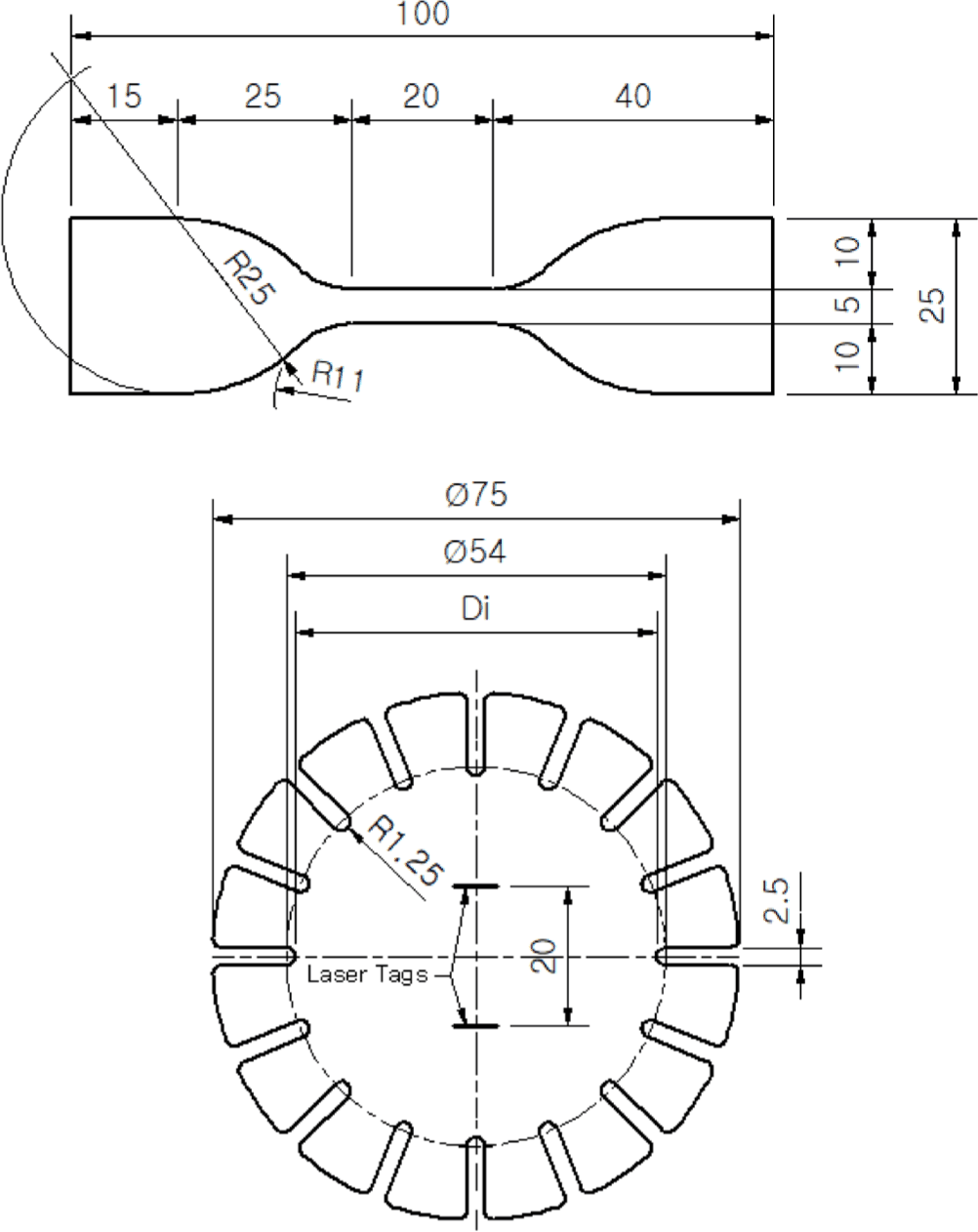
The uniaxial tensile test was conducted to realize a state of uniaxial deformation without constraint in the width and thickness directions of the specimen. A dumbbell-shaped specimen was used in this study. The specimen was stretched in the longitudinal direction so that the reduction of cross-sectional area could occur freely, and the deformation gradient tensor F and the nominal stress tensor P were expressed as
Where λ the principal stretch, P is the tensile load, and A0 is the initial cross-sectional area.
This test was performed using a circular specimen to realize an equibiaxial deformation state in which identical strains are applied in two orthogonal in-plane directions. The deformation gradient tensor F and the nominal stress tensor P were expressed as
Where λ the principal stretch, P is the tensile load, and A0 is the initial cross- sectional area.
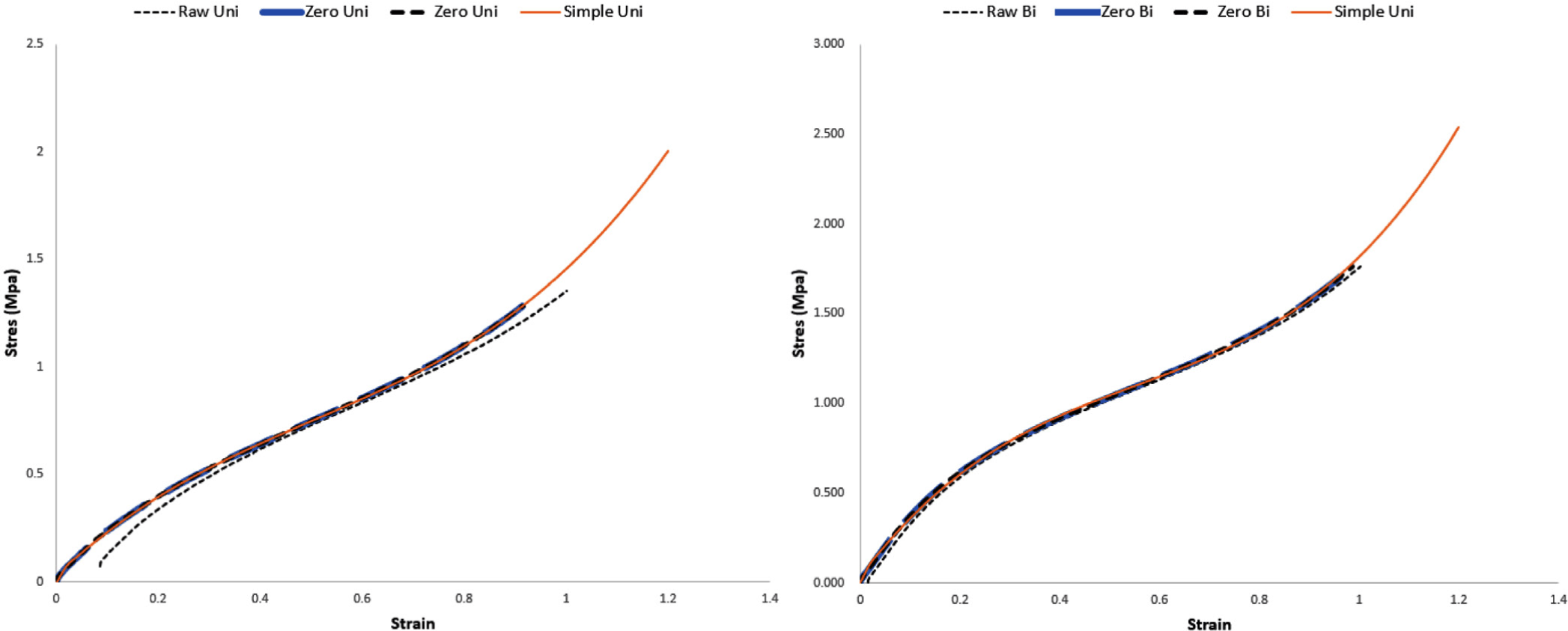
In this study, three datasets, raw data, zero-setting data and simply preprocessed data, were constructed based on the curves obtained from uniaxial and equibiaxial tensile tests. The raw data contained initial load offsets and noise. The zero-setting data were generated by aligning the starting point of the stress-strain curve to (0, 0) in order to remove the initial offset of the raw data. In this study, zero-setting was applied as a simple origin shift, and no elasticity-theory-based correction was used. The simply preprocessed data were obtained by interpolating the strain at uniform intervals (Δε=0.02), thereby ensuring the monotonicity and continuity of the curve. The overall differences among the raw data, zero-setting data and simply preprocessed datasets are summarized in Figure 2. Although the three datasets appear similar in Figure 2, differences in the initial offset and strain spacing can still influence the numerical stability of Ogden fitting. In particular, the simply preprocessed data has uniform strain intervals and maintains monotonic behavior over a wider strain range compared to the other datasets.
These preprocessed datasets were then used with Abaqus Evaluate and Marc Experimental Data Fit to obtain the third-order Ogden model coefficients (μi, αi). Because Abaqus Evaluate does not impose any sign constraints on the coefficients, negative coefficients were obtained for some datasets, which led to Stability limit warnings2 and non-physical stress growth. In contrast, Marc provides a Positive Coefficients option3, which enforces sign constraints and thus maintains physically reasonable combinations of coefficients.
In addition, to enable the derivation of Ogden coefficients even in environments where commercial analysis software is not available, a simplified third-order Ogden fitting procedure using Microsoft Excel Solver was constructed for simply preprocessed data. The six third-order Ogden coefficients (μ1, μ2, μ3, α1, α2, α3) were treated as optimization variables, and the objective function was defined as the weighted sum of squared errors between the nominal stress predicted by the Ogden model and the preprocessed stress data. The simply preprocessed strain data were entered into the spreadsheet, and the nominal stresses at each strain point were calculated from the third-order Ogden stress equations for uniaxial and equibiaxial deformation. Different weighting factors were assigned across the strain range so that the fitting process could reflect not only the initial response but also the nonlinear and high-strain behavior. Excel Solver then adjusted the six coefficients iteratively until the residual error no longer decreased. Positive constraints were imposed on all coefficients during the optimization. The Microsoft Excel-based coefficients obtained in this way were applied to Y-and Z-direction bush analyses for a preliminary comparison with the coefficients derived from commercial solvers.
The Ogden coefficients obtained from each preprocessing– solver combinations are summarized in Table 1.
The third-order Ogden hyperelastic coefficients derived in this study were implemented into a finite element model of the 4-bridge type rubber bush to examine the product-level behavior and the convergence characteristics of the analysis. The simulations were performed using the implicit procedure in Abaqus, and the element types and node counts used in the model are summarized in Table 2.
| Number of Elements & Nodes | |
|---|---|
| Nodes | 57,593 |
| Elements | 46,240 |
| Element type | |
|---|---|
| Outer Pipe | C3D8 |
| Rubber | C3D8H |
| Inner RP | RNODE3D |
The inner metal part was idealized as a rigid body using a reference point and subjected to displacement-controlled loading, while the outer metal part was constrained with fixed boundary conditions. General Contact was used to define the contact conditions, and the friction coefficient was set to 0.3. The analyses were carried out by applying Y- and Z-direction displacement boundary conditions identical to those in the experiments, and the results were obtained in the form of Load–Displacement curves.
To verify the product-level validity of the Ogden coefficients obtained from specimen tests, load–displacement tests were conducted on a 4-bridge type rubber bush. The tests were performed using a dedicated rigid jig, in which displacement was applied to the inner metal part while the outer metal part was fixed.
The X-direction test was carried out only within an almost linear region due to the structural characteristics of the product; since it is not directly relevant to the objective of this study, which is to analyze differences in nonlinear behavior, it was excluded from the subsequent analysis.
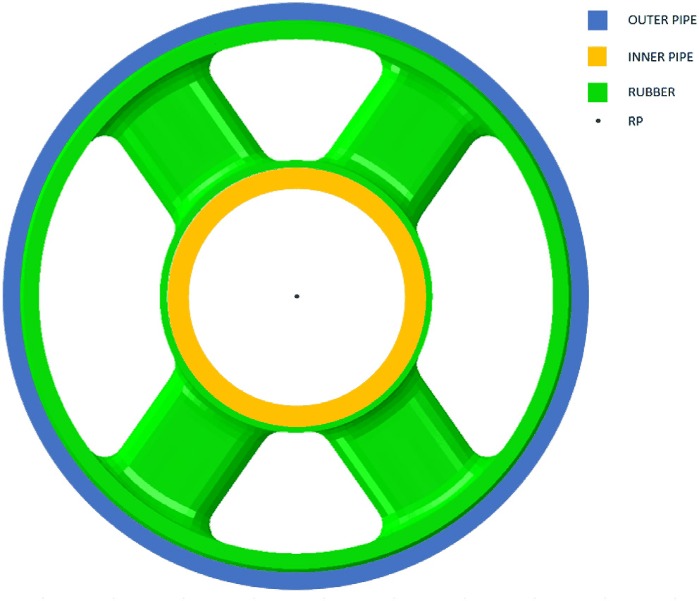
For the Y- and Z-direction tests, tension and compression were each applied up to a maximum displacement of 13 mm, and the loading cycle was repeated twice in order to capture the nonlinear characteristics of the bush. The detailed geometry of the 4-bridge rubber bush and the definitions of the loading directions are illustrated in Figure 3.
Results and Discussion
In this study, the Ogden coefficients obtained from the raw data, zero-setting data and simply preprocessed dataset and their combinations were implemented in product-level analyses, and the resulting load–displacement responses were compared with the experimental results. The comparison was made with a particular focus on the effect of preprocessing on the convergence behavior of the analyses.
The stability of the Ogden coefficients for each preprocessing scheme was evaluated using the stability limit function in Abaqus Evaluate. For the raw data, stability limit warnings appeared due to initial load offsets and noise. The zero-setting data exhibited a stable response in the initial region; however, as the strain increased, it clearly became unstable and was flagged as “Unstable” at higher strain levels. In contrast, the simply preprocessed data, which were generated by uniform-interval interpolation, maintained monotonicity over the entire strain range and were consistently judged as “Stable” in the Evaluate procedure.
Because Abaqus Evaluate does not provide sign constraints on the coefficients, the non-uniform strain spacing of the zero-setting data caused slope fluctuations in the high-strain region. On the other hand, Marc Experimental Data Fit, with the Positive Coefficients constraint, produced stress curves that were smoother and more physically consistent even under the same preprocessing conditions. In particular, the Marc program with simply preprocessed data combination yielded parameters that ensured both preprocessing stability and numerical robustness.
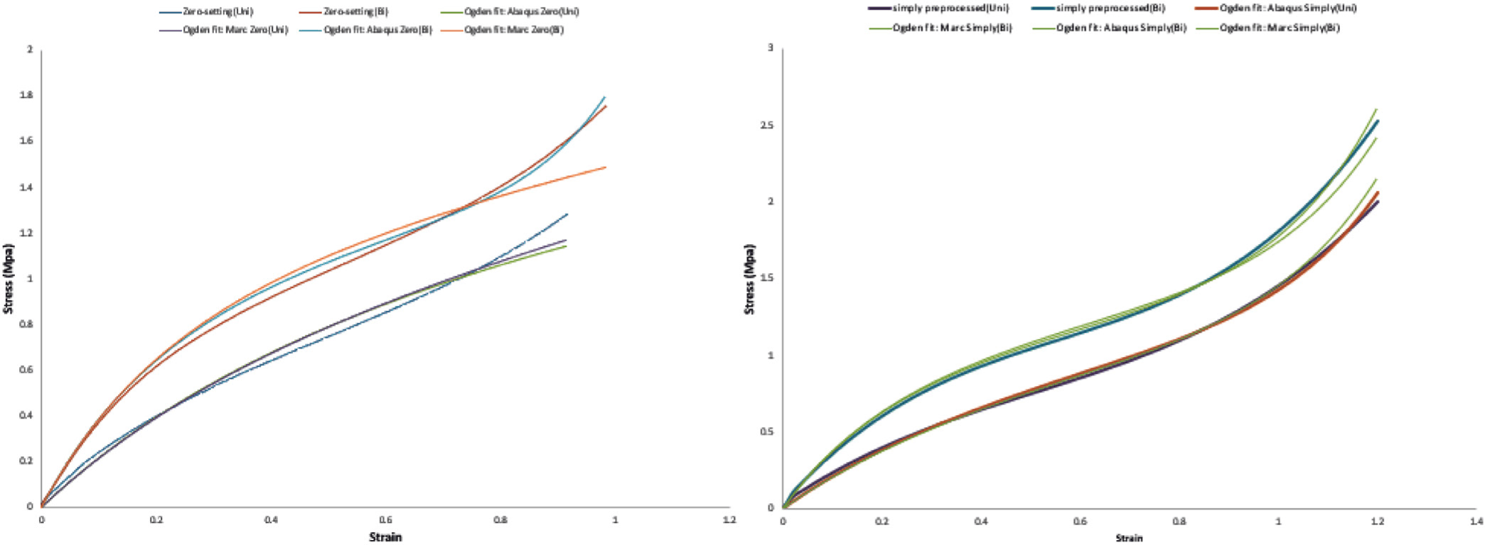
The raw data, which lacked numerical stability, were excluded from the stress–strain curve comparison. The stress–strain curves reconstructed from the derived Ogden coefficients showed that the simply preprocessed data-based coefficients reproduced the preprocessed data almost exactly in uniaxial deformation. The corresponding comparisons between the fitted curves and the preprocessed datasets are summarized in Figure 4.
The Y-direction product-level analysis results for the four parameter combinations are shown in Figure 5.
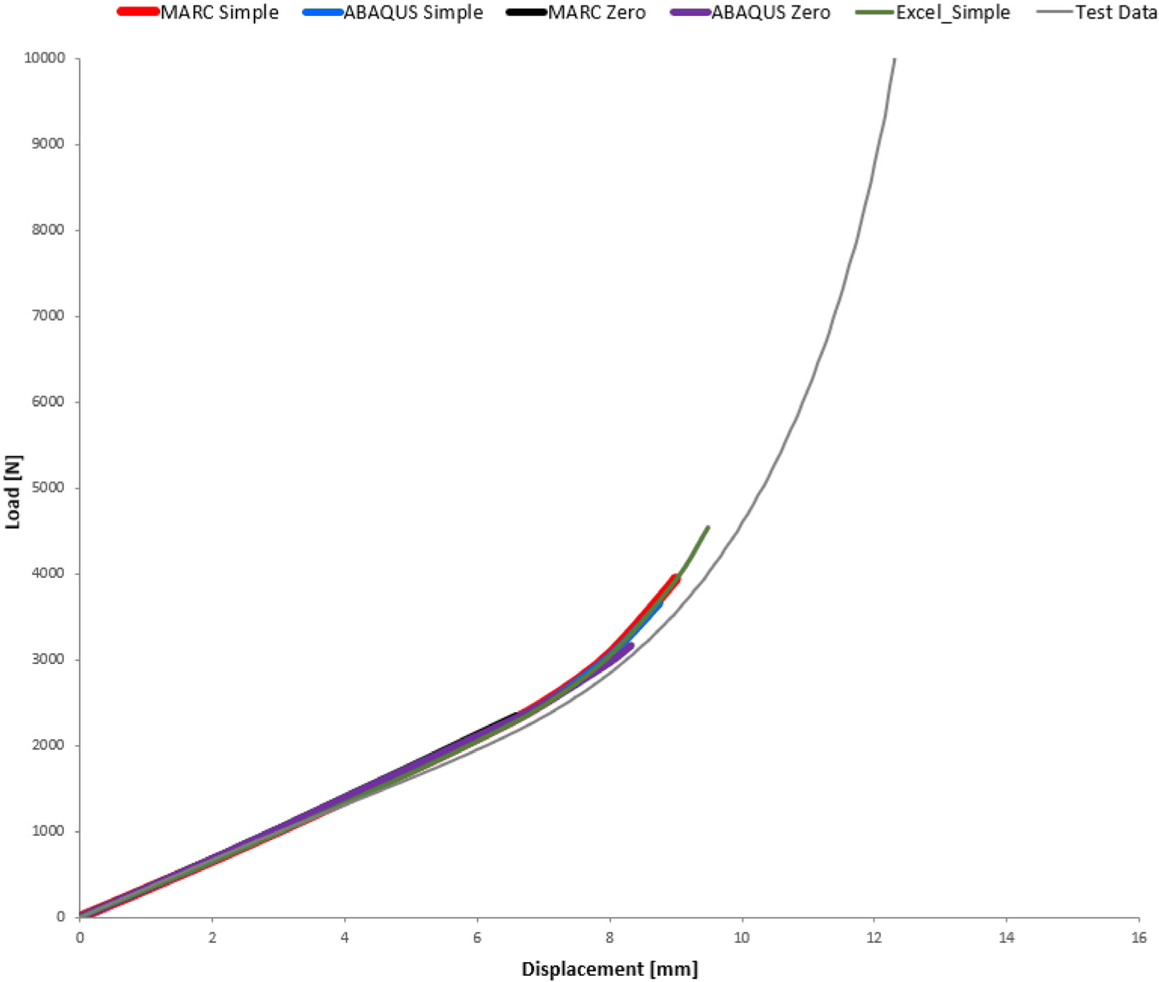
In the linear region, all analyses exhibited a slope similar to that of the test curve; however, beyond approximately 6 mm, clear differences appeared in both the convergence range and load level. The analysis using the Marc program with simply preprocessed data coefficients remained stable up to about 9 mm, reaching a maximum load of approximately 3.9 kN and thus covering the widest nonlinear region. The Abaqus program with simply preprocessed data converged up to about 8.8 mm, reproducing part of the early nonlinear region. In contrast, the Abaqus program with zero-setting data and the Marc program with zero-setting data terminated prematurely at about 8.3 mm and 6.6 mm, respectively, indicating that the zero-setting data were less capable of tracking the nonlinear Y-direction behavior than the simply preprocessed data.
The Z-direction product-level analysis results for the four parameter combinations are presented in Figure 6.
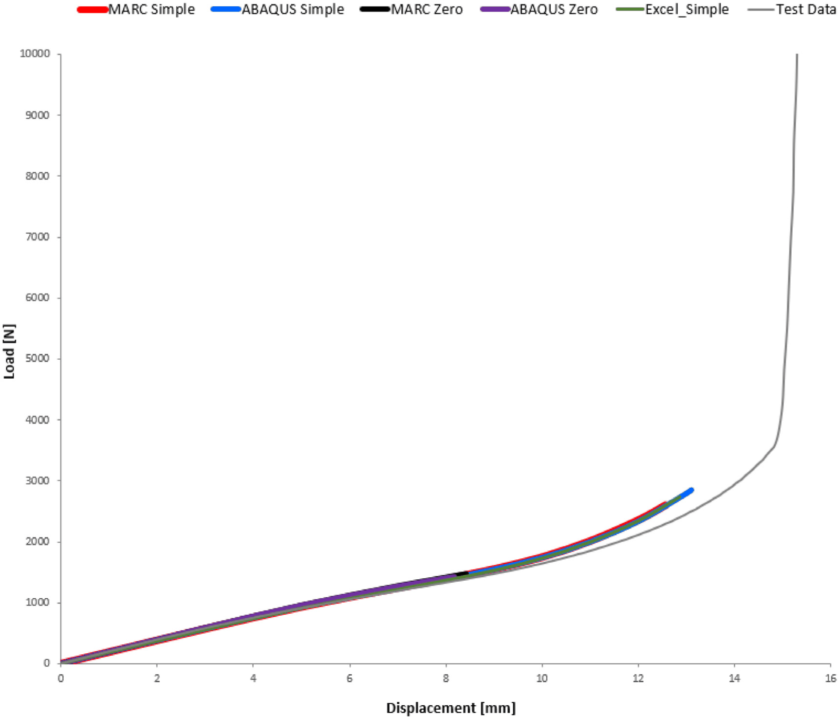
In the initial linear region, all four combinations showed slopes comparable to the experimental results, but as the displacement increased, distinct differences emerged in both load level and the displacement at which convergence was lost. The analysis using the Abaqus program with simply preprocessed data coefficients remained stable up to approximately 13.3 mm and 2.6 kN, exhibiting the best convergence among the four combinations. The Marc program with simply preprocessed data also converged up to about 12.5 mm and captured the nonlinear behavior sufficiently, although its maximum load and displacement were slightly lower than those of the Abaqus program with simply preprocessed data. In contrast, both the Marc program with zero-setting data and the Abaqus program with zero-setting data failed during the stage where the load rose steeply in the nonlinear region, showing relatively poor convergence.
Although the shear modulus values calculated from the Ogden coefficients differed among the parameter sets in Table 1, the product-level responses were similar in the initial loading region. The differences became more evident in the nonlinear region, mainly through the convergence range and load level.
Additionally, when the coefficients obtained from Excel Solver for the simply preprocessed data were applied to the product-level analyses, the overall trends of the load– displacement curves in both the Y and Z directions were similar to those of the simple–Marc combination. These results were used as a preliminary assessment of the potential applicability of the lightweight fitting procedure in environments where commercial solvers are not available.
Conclusions
In this study, preprocessing datasets were constructed from tensile-test raw data, third-order Ogden hyperelastic models were derived from these datasets, and the resulting models were applied to FE analyses. Compared with the raw data, zero-setting data and simply preprocessed data showed more stable behavior and improved convergence at both specimen and product levels. For the bush and loading conditions examined in this work, the analyses based on simply preprocessed data exhibited a wider and more stable convergence range than those based on zero-setting data in both the Y- and Z-directions, regardless of whether Abaqus or Marc was used. Although some differences in the detailed convergence range and load–displacement response were observed between the two commercial solvers due to their internal implementations, the overall tendency that simple-based Ogden fitting is more robust than zero-setting data for the present rubber bush application remained consistent.
Furthermore, considering environments in which commercial analysis software is not available, a trial Excel Solver–based lightweight Ogden fitting procedure was developed for the simply preprocessed data, and it was confirmed that the resulting product-level analyses can reproduce tendencies similar to those of the Marc program with simply preprocessed data combination. However, because no detailed stability evaluation or quantitative specimen-level error analysis was performed for the Excel-based coefficients, the reliability verification and automation of this lightweight fitting procedure remain topics for future work.

